Background
Before we jump into looking if our time series are stationary or not. Firstly, we need to understand what it means and why it is important.
What does stationary time series mean? It simply means that its joint probability distribution is time-invariant. In a regression model, the ordinary least squares (OLS) estimators are not consistent for non-stationary series and the standard statistical tests are not valid. Meanwhile, many of statistical tests assume that the data is stationary. Therefore, making it very important to consider when doing some data analysis.
Testing for unit root in Python
There are a many unit-root and stationarity tests available. However, here, I will focus on the most popular one unit root test, i.e. Augmented Dickey-Fuller ('ADF'). However, you may wish to also try Phillips-Perron ('PP'), and for checking the stationarity, Kwiatkowski-Phillips-Schmidt-Shin ('KPSS'). ADF and PP tests test a null hypothesis that the process contains the unit root against the alternative that the process in weakly stationary. Whereas the KPSS test tests the null hypothesis of the process being weakly stationary against the alternative that the process contains a unit root.
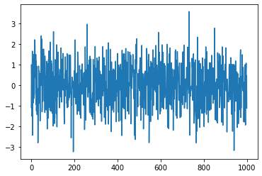
To begin with, let us create a time series:
> import numpy as np
> import matplotlib.pyplot as plt

> np.random.seed(seed=123)
> mean, standard_dev = 0, 1
> errors = np.random.normal(mean, standard_dev, 1000)
> y_1 = []
> for i in range(0,1000):
>     y_1.append(errors[i])
> plt.plot(y_1)
To test this series we run the following code:
> from arch.unitroot import ADF
> print(ADF(y_1, method = 'bic', trend='c'))
    Augmented Dickey-Fuller Results
    =====================================
    Test Statistic                -31.923
    P-value                         0.000
    Lags                                0
    -------------------------------------

    Trend: Constant
    Critical Values: -3.44 (1%), -2.86 (5%), -2.57 (10%)
    Null Hypothesis: The process contains a unit root.
    Alternative Hypothesis: The process is weakly stationary.
Since the p-value is very small, there is enough statistical evidence to reject the null hypothesis that the process contains a unit root. Therefore, the results point on the corresponding series being weakly stationary.
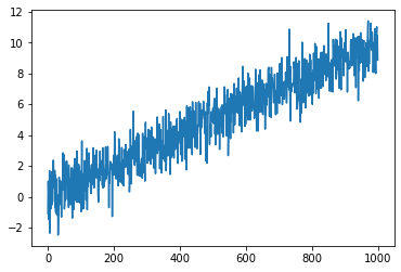
For trending series:
> x = np.arange(0, 10, 0.01)
> y_2 = []
> for i in range(0,1000):
>    y_2.append(x[i]+errors[i])
> plt.plot(y_2)
> print(ADF(y_2, method = 'bic', trend='c'))
    Augmented Dickey-Fuller Results
    =====================================
    Test Statistic                 -0.746
    P-value                         0.834
    Lags                               11
    -------------------------------------

    Trend: Constant
    Critical Values: -3.44 (1%), -2.86 (5%), -2.57 (10%)
    Null Hypothesis: The process contains a unit root.
    Alternative Hypothesis: The process is weakly stationary.
Here, since tending series were not taken into consideration, the test failed to reject the null hypothesis. This result indicates that the series may be non-stationary. This makes sense, since only a constant component was allowed for, and these series cointains a linear trend, and so the mean is not time invariant. Let us fix this by including a constant and linear time trend.
> print(ADF(y_2, method = 'bic', trend='ct'))
       Augmented Dickey-Fuller Results
    =====================================
    Test Statistic                -30.829
    P-value                         0.000
    Lags                                0
    -------------------------------------

    Trend: Constant and Linear Time Trend
    Critical Values: -3.97 (1%), -3.41 (5%), -3.13 (10%)
    Null Hypothesis: The process contains a unit root.
    Alternative Hypothesis: The process is weakly stationary.
After taking away this linear trend the null hypothesis can indeed be rejected.
> from arch.unitroot import ADF
> print(ADF(y_1, method = 'bic', trend='c'))
       Augmented Dickey-Fuller Results
    =====================================
    Test Statistic                -31.923
    P-value                         0.000
    Lags                                0
    -------------------------------------

    Trend: Constant
    Critical Values: -3.44 (1%), -2.86 (5%), -2.57 (10%)
    Null Hypothesis: The process contains a unit root.
    Alternative Hypothesis: The process is weakly stationary.